How to Make a Bell Curve in Google Sheets {Easy Guide}

Charts and graphs are a great way to visualize the data in your spreadsheet. Thankfully, Google Sheets provides a powerful set of tools to make this possible. One great way is to use the Google Sheets distribution chart. Commonly known as a bell curve graph. To create this, we need to use the normal distribution of the data.

Creating a bell curve chart can help you better understand your data. This helps you know where the most data points lie in the chart, how close the relationships between the points are, and which data points are considered outliers. In this article, we’ll explain what a bell curve is, why we use a bell curve, and how to create a normal distribution curve in Google Sheets.

Learn how to create a bell curve in Google Sheets in a few easy steps.

What Is a Bell Curve?

Bell curve charts, also known as normal distribution charts, are commonly used to analyze financial data in statistics. The lines produced in this graph are usually symmetrical curves in the shape of a bell, hence the name.

The highest part of the curve shows the mean, median, and mode of the data and is the densest part of the graph. The width of the curve indicates the standard deviation around the mean.

The data usually follow the 68/95/99.7 rule of the bell curve. Here, 68% of the information is within 1 standard deviation of the data mean. 95% of the data are within 2 standard deviations of the mean and 99.7% of the data are within 3 standard deviations of the mean.

Examples of bell curves are often found in real life. Take for example the height of the students in your class. We can conclude that most students are close to the mean of the dataset, but some students are slightly below or slightly above the mean. On a bell curve, this is to the left and right of the curve’s highest point.

Why You Should Use a Bell Curve

Bell Curve Google Sheets charts aren’t just used in the financial world to analyze stocks or showcase real estate values. It can also be used in everyday situations like visualizing classroom grades, reviewing product scores, etc., and generally for data groups with dense values ​​close to the mean of the data set.

These charts can help you decide if a stock is safe to invest in. We can also offer fair prices for real estate. These are also useful for comparing review scores, as their averages are usually near the middle of the scale, giving you a clearer idea of ​​whether you should buy the product.

For example, on a review score scale of 1 to 10, if most reviews are around 8, 8 is the highest point on the bell curve and others are lower. Suppose there is a minority who rated the product as 3. In that case, it could be considered an outlier, meaning it cannot be considered reliable.

How to Make a Bell Curve in Google Sheets

Creating a bell curve works similarly to creating the best line for a scatterplot in Google Sheets. But before we create the bell curve for Google Sheets, let’s talk about the dataset we’ll be using. The example spreadsheet below contains exam scores for 15 students.

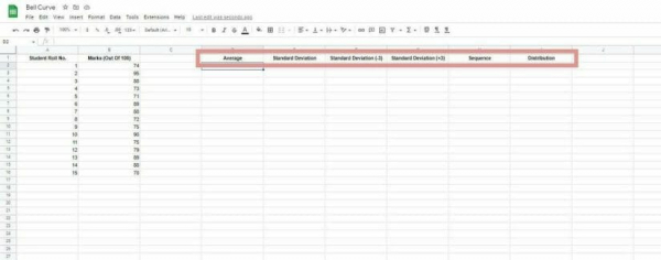
The first thing we need to do is add columns to our spreadsheet. These are the mean, standard deviation, standard deviation +3, standard deviation -3, order and distribution.

First, we need to calculate the mean (mean). This can be done using the AVERAGE formula. To do this, follow these steps:

1. Click on the cell where you want to enter the formula (in this example D2 under the title “Average).
2. Enter the beginning of the formula =AVERAGE
3. Please enter a range. In this case the cell range B2:B16
4. Add a closing parenthesis to end the formula
5. Press Enter to run the formula

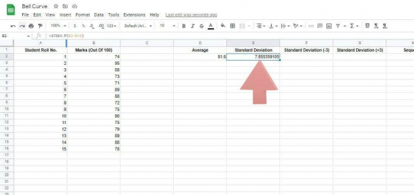
Now let’s use the STDEV.P formula to find the standard deviation of the data. This can be done using the same steps as above.

The formula used to find the standard deviation in this case is:

=STDEV.P(B2:B16)

Notice that the range does not change. This is important for building an accurate bell curve.

Next, calculate the values ​​for standard deviation -3 and standard deviation +3. To find the value for standard deviation -3, multiply the standard deviation by 3 and subtract it from the mean. For +3 standard deviations, multiply the standard deviation by 3 and add it to the mean.

The formula used here is:

• Standard Deviation (-3): =D2-(E2*3)
• Standard Deviation (+3): =D2+(E2*3)

Then I need to display the numbers for the entire sequence. It is used to plot graphs.

The formula used to do this is:

 =SEQUENCE(G2-F2+1,1,F2)

This function simply fills an ordered list of numbers based on the parameters provided.

The last column contains the distribution of the data. To do this, use the ARRAYFORMULA and NORM.DIST formulas. The syntax for the entire formula is:

=ARRAYFORMULA(NORM.DIST(range, mean, SD, FALSE))

Building a Bell Curve in Google Sheets

Now that we have the data we need, let’s create a bell curve. Here are the steps:

1. First, highlight the data in the Sequence and Distribution columns
2. Click “Insert” in the top bar
3. In the dropdown menu, click Chart
4. A chart editor will appear on the right side of the screen
5. Select line chart as chart type

Customizing the Standard Deviation Graph in Google Sheets

Optionally, you can customize the appearance of the bell curve chart.

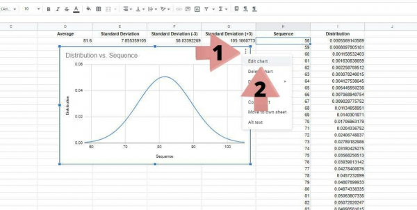
To do this, we need access to the chart editor do this:

1. Click on the three dots icon in the upper right corner of the chart.
2. Click Edit Graph. This will open the chart editor on the right side of the screen.
3. In the chart editor, click Customize. This will bring up another window where you can change the appearance of the graph.

There are various sections here. You can change options such as background color, font, title text, line color and opacity. When you have finished customizing the graph to your liking, click the cross symbol to close the graph editor. This will save your changes.

FAQ

How Do You Make a Bell Curve in Google Sheets?

To create a standard deviation chart in Google Sheets, you first need to find the mean and standard deviation of your data. Next, calculate the values ​​for standard deviation -3 and standard deviation +3. From there, create a sequence from the lowest value to the highest value in the dataset. Find the distribution of data within a value. Once you have this data, use the spreadsheet’s charting features to create a line chart. This gives the shape of a bell curve.

How Do You Construct a Bell Curve? / How Do I Create a Curved Trendline in Google Sheets?

1. Once you have the values ​​you need to create the bell curve, select values ​​for Order and Distribution.
2. There, click Insert and then click Chart from the dropdown menu.
3. Select Line Chart in the Chart Type section of the Chart Editor

 Trend Lines: How to Add Optimal Lines to Google Sheets

Wrapping Up the Bell Curve

Creating a bell curve requires many steps and finding some initial data points. However, the end result is worth the struggle.

Pay close attention to the size of the curvature when creating the bell curve. A tall and narrow curve means that the standard deviation is small, meaning that the data are not very scattered. A short but wide curve represents a significant standard deviation, meaning the points are spread out further.

I hope this article has helped you better understand how to create a bell curve in Google Sheets. If you want to learn more about creating charts in Google Sheets, check out these guides: