Google Sheets QUERY With Multiple Criteria (2 Easy Examples)

Google Sheets has extensive search and filter capabilities. However, the QUERY function is often the most powerful. Unfortunately, it can be a little difficult to use. You may be wondering, “Can Google Sheets query multiple criteria?” The short answer is yes. This guide will show you step by step exactly how to do that. If you want to know more, read on.

What Is the Google Sheets Query Function?

The QUERY function in Google Sheets allows you to apply queries to datasets. You can extract subsets of your data from the main dataset, allowing you to explore areas of interest within your data and gain a deeper understanding.

Queries can be thought of like filters or pivot tables. If you have used SQL to interact with databases before, you will recognize the similarity of the format of the QUERY function. Essentially, the QUERY function mostly uses Google Sheets to perform SQL-style queries against a given dataset.

The Syntax for Google Sheets QUERY With Multiple Criteria

Before we look at the QUERY function in action, let’s take a quick look at how the formula works. QUERY has the following syntax:

=QUERY(data, query, header)

The parameters of the multi-conditional query function in Google Sheets are:

1. data: This parameter defines the range of cells to query. Each column of data can hold numeric, Boolean, or string values. These can include time and date. If you have mixed-type data in a column, the majority data type determines the data type of the entire column in your query. A small number of data types are considered null values.
2. query: This parameter defines the query to run on the data. It is written in Google’s Query Visualization API language. Query values ​​must be quoted or be cell references containing the appropriate text.
3. header: This is an optional parameter used to define the number of header lines towards the beginning of the data. If you omit this parameter or set it to -1, the value is approximated based on the contents of the data parameter.

How Do Logical Operators Work?

Logical operators are symbols or words used to create connections between expressions, and the value of the compound expression created depends on the value of the original expression and the meaning of the operators used.

Commonly used logical operators include OR, AND, and NOT.

In many languages, boolean data values ​​consist of two groups. The first group contains relational operators and the second group contains logical operators in expressions. Test expressions that control program flow are constructed using logical operators, also known as Boolean expressions.

Three common logical operators modify another boolean operand to produce a boolean value these are:

1. AND: This operator requires both terms to appear in all returned values. If one term appears in the document and the other does not, the term is excluded from the list. This operator is typically used to narrow your search. For example, searching for “Google Sheets AND Microsoft Excel” will return results containing both the Sheets and Excel search terms.
2. OR: This operator requires exactly one term to appear in the returned value. For example, searching for the keywords “ecology OR pollution” guarantees that your search results will include the terms ecology, pollution, or both.
3. NOT: This operator removes all instances of the term from the search. For example, searching for “not malaria” guarantees that the search results will not contain the term malaria.

How to Use Query Multiple Criteria Google Sheets

Now you know how the QUERY function works in spreadsheets. Let’s look at some ways to use this in Sheets.

Google Sheets QUERY AND

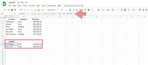
in this example, we have data for several businesses, showing their categories and revenue. You want to know which companies in the food category have made a profit of $60,000 or more. Both conditions must be true, so we use AND as the logical operator.

Here’s how to use AND in your QUERY with multiple criteria in Google Sheets:

1. Click the cell where you want to enter the formula.
2. Enter the first part of the QUERY expression. First, enter the equals (=) sign. This tells Google Sheets that the following text is part of the formula. Create a QUERY here and add a left parenthesis.
3. Then you have to enter the first parameter, the data. In this example, the cells are A2:C7.
4. Add a comma (,) to separate the parameters.
5. Then enter the second parameter, the query. Use the following logical expression: “Select A, B, C where B contains ‘Food’ and C>60000”. Be sure to add the quotation marks. Otherwise Google Sheets will return #ERROR!
6. Add a closing parenthesis to the end of the formula and press Enter.

Google Sheets will return values ​​that meet all the criteria you specify. As you can see in the screenshot above, it shows food businesses that have made over $60,000 in revenue.

Google Sheets QUERY OR

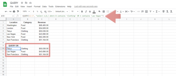
Using the same data, I would like to find either businesses in the clothing category or businesses located in Las Vegas. An OR query is satisfied if either condition is met. Basically follow the same steps used in the previous example. However, the query operators are changed according to your requirements.

The formula used to do this is:

=QUERY(A2:C7, “Choose A, B, C. B contains ‘Clothing’ OR A contains ‘Las Vegas’”)

Most of the formulas used here are the same as those used in the previous example. The only exception is query parameters.

Explanation of How It Works

Let’s break this down and explain what each part of the parameter means:

• select A, B, C – This part of the parameter specifies the columns to select.
• Where B contains “Clothing”. This is the first condition to check, which is specified to search for the keyword “Clothing” in column B.
• OR – This is the logical operator used.
• A contains “Las Vegas”. This is the second condition to check, which is specified to search for the keyword “Las Vegas” in column A.

Related reading: How to use lookups in Google Sheets

Frequently Asked Questions

How Do I QUERY a Condition in Sheets?

The QUERY function in spreadsheets is used to set conditions to find the data you are looking for specifically. It works as a filter to some extent. A query searches columns in a spreadsheet for values ​​that match your criteria and displays the results.

The function syntax is =QUERY(data, query, header).

it requires three parameters to work. The data parameter defines the range of cells to query. Query parameters define the query to run on your data and are written by Google in the Query Visualization API language headers is an optional parameter used to specify the number of header rows at the beginning of the dataset.

Can You Filter by Multiple Conditions in Sheets?

If your Google Sheets query contains multiple conditions, you can use a QUERY expression in Sheets to apply many conditions to your dataset using logical operators. This can be done using Google’s Query Visualization API Language. Queries are written in a statement-like format and allow you to specify conditions to apply to your data using AND, OR, and NOT operators. When executed, the spreadsheet will display the results in the cell where you ran the formula.

Wrapping Up

I’m glad you answered the question, “Can Google Sheets query multiple criteria?” Learning the exact phrases to write in the Query Visualization API Language can take some time, but learning the operators is a good start. If you have any questions, let us know in the comments. Or see related content for more information.