2023 Guide to the Powerful IMPORTHTML Google Sheets Function

The IMPORT function is one of the best functions to save time when working with large amounts of data from external sources. The IMPORTHTML Google Sheets feature is the most useful as it allows you to retrieve data from websites quickly and easily.

This guide provides simple step-by-step instructions on how to use the IMPORTHTML function. Also a quick look at some of his other IMPORT functions for Google Sheets. This will make it easier to tackle this function in the future when you come across it.

For a complete overview of IMPORTHTML and the IMPORT function in Google Sheets, read this article.

What Is HTML?

HTML or Hypertext Markup Language is used to create web pages. This language describes the structure of web pages. A developer uses the HTML language to design the interface through which the browser displays her web page elements such as text, media, and hyperlinks.

HTML is often used to add hyperlinks, so users can use HTML to navigate and insert links. The language also allows you to format and organize your documents in a similar way to Google Docs.

What Is the Google Sheets Import Data From Website Function?

The Google Sheets IMPORTHTML function allows you to search and extract data from an HTML table or list. This function is intended to be used to retrieve a list or table from an external website. Before explaining how to use the Google Sheets web data import formula, let’s take a look at its format. The formula is:

=IMPORTHTML(url, query, index)

This formula requires three parameters to be entered these are:

1. URL: This parameter defines the URL of a web page or a reference to a cell containing a URL. This address should include the protocol, such as http://. If you enter the URL value directly into the expression, be sure to enclose it in quotation marks.
2. Query: This parameter defines whether the data is in list or table format, depending on what kind of data you are importing into the spreadsheet.
3. Index: The index parameter defines the table or list to import into the spreadsheet. Tables and lists are maintained with separate indexes. In other words, if both the list and the table exist on the page, the index can be 1.

How to Use IMPORTHTML in Google Sheets

Google Sheets Import Table From Website

In this example, we want to get a table of the list of highest-paid movie actors from the Wikipedia page. Doing this manually takes a lot of time and effort, so we use the HTML import feature in Google Sheets.

Here’s how to get a table using IMPORTHTML in Google Sheets:

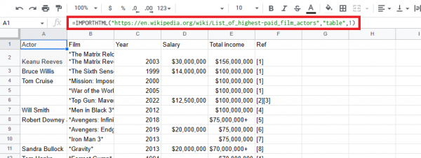
1. Click the cell where you want to import data. The top left element of the table will be imported into the cell containing the formula. Make sure you have free space to import the table properly.
2. Enter the first part of the IMPORTHTML function in Google Sheets (=IMPORTHTML(.
3. Enter the first parameter. This defines the URL containing the table to import. In this case, enter “https://en.wikipedia.org/wiki/List_of_highest-paid_film_actors”. Include the quotes if you add the URL directly to the expression.
4. Add a comma to separate the parameters.
5. Then add a second parameter, the query. In this example, we want to import a table, so we write the parameter as “table” including the quotes. Add another comma to separate the parameters.
6. Now add the final index parameter. This defines the table number to import into the spreadsheet. In this case, we write 1 because it is the first table on the web page.
7. Add a closing parenthesis to end the formula and press Enter to run the formula.

Import List From Website Into Google Sheets

If you have a list on a web page, you can import it into Google Sheets using the same steps you would use to import a table. Here’s how to get a list from a website and import the HTML into Google Sheets:

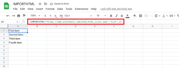
1. Click the cell where you want to import the data and enter the first part of the Google Sheets IMPORTHTML function (=IMPORTHTML(.
2. Enter the URL parameters. In this case it is “https://www.w3schools.com/html/html_lists.asp”. Be sure to add the quotation marks. Add commas to separate parameters.
3. Then add query parameters. In this example, we want to import a list, so we write the parameter as “list”, including the quotes. Add another comma to separate the parameters.
4. Enter the index parameter here. In this case it is 2.
5. Finally, add a closing parenthesis to end the formula and press Enter to execute the formula.

Using Cell References with IMPORTHTML

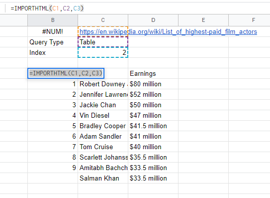
You can also use cell references as parameters for the IMPORTHTML function. The example below uses the following formula:

=IMPORTHTML(C1,C2,C3)

Instead of entering URLs, queries and indexes into formulas.

Import Specific Rows and Columns

To import only certain rows and columns using IMPORTHTML, simply specify it within the INDEX function: In the example below I used the following formula: =INDEX(IMPORTHTML(“https://en.wikipedia.org/wiki/List_of_highest-paid_film_actors”,”table”,2),3,2)

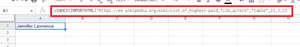
You’ll notice the ,3,2) outside the first closing bracket. This tells the INDEX function to get the data from row 3 and column 2.

Reasons Why the IMPORTHTML Function Isnt Working

If the formula executes correctly, the list or table will appear within seconds. However, if you don’t see any data or get an error prompt, it could be for one of the following reasons:

• URL changes: If the URL of the table or list you’re importing has changed and has been moved to a different URL, double-check the URL.
• Protocol changes: Redirects to websites often cause problems with IMPORTHTML expressions. Make sure the protocol is http or https for the formula to work properly.
• Index changed: You may find that Google Sheets imported the wrong table or list. A possible reason for this is that the list or table index has changed. To fix this issue, try moving up and down until the table loads properly.
• Scraping blocked: The website owner may have blocked the use of bots or scrapers to stop scraping of web content.

Google Sheets Web Scraping: A Simple Guide for 2023

How to Get Indexes of Tables/Lists to Pull Data From Website to Google Sheets Using IMPORTHTML

1. In your browser, go to Settings > More Tools > Developer Tools.
2. Click on the Console tab
3. Copy the following code into the text box:

Variable index = 1; .forEach.call(document.getElementsByTagName(“table”), function(elements) { console.log(“Index: ” +index++, elements); });

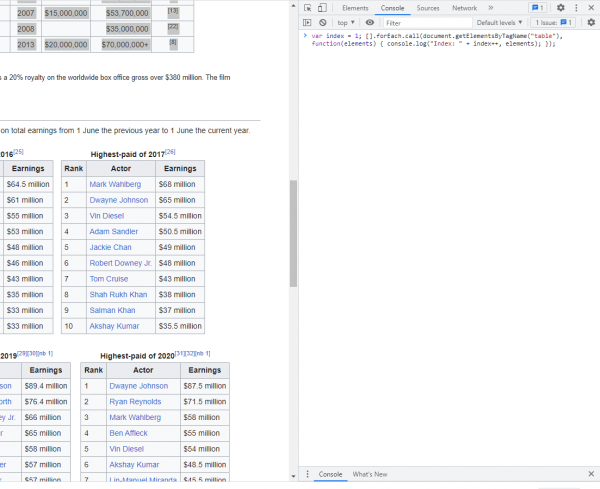
1. Press enter
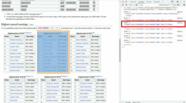
2. Hover your mouse over the option until the table you want to import is highlighted.
   

   

if you want to import a list instead, you should use “ul,ol” as arguments instead of “table” like this:

Variable index = 1; .forEach.call(document.getElementsByTagName(“ul,ol”), function(elements) { console.log(“Index: ” +index++, elements); });

How to Set a Custom Interval for Refreshing Your Imported Data

You can use a combination of Add Query and Google Apps Script to change how often your imports are updated.

1. Add “update” to cell A1 and number 1 to cell B1
   

   

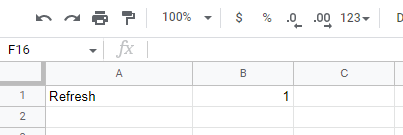
2. Use the same formula as usual, but concatenate the query parameter and refresh cell in the URL argument. For example, for the site used above:

=(IMPORTHTML(“https://en.wikipedia.org/wiki/List_of_highest-paid_film_actors” & “?refresh=” & B1,”table”,1)

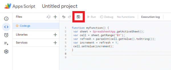
1. Go to Extensions > App Scripts
2. Copy and paste the following code into the text box:

function myFunction() { varsheet = SpreadsheetApp.getActiveSheet(); var cell =sheet.getRange(“B1”); varfresh = parseInt(cell.getValue().toString()); var increment = refresh + 1; (increment); }

1. Click the floppy disk icon to save the script.
   

   

2. Open “Triggers” in the left menu and go to “Add Trigger
3. Under Select Event Source, select Time-Driven
   

   

4. Select the appropriate option from the two drop-down lists below and click Save.
5. Back in the editor window, click Run
   

   

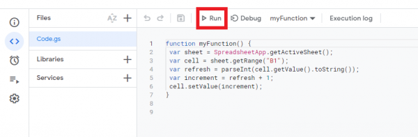
6. The data will be updated at the specified interval.

Similar Options for Scraping Data Into Google Sheets

Several other functions can be used to bring content into Google Sheets. Let’s take a look at some of them.

IMPORTXML

XML is a markup language similar to HTML. However, there is one important difference. XML has no predefined tags. Alternatively, you can define your own tags to meet your needs. The IMPORTXML function in Google Sheets allows you to bring XML into your spreadsheet.

The formula syntax is:

=IMPORTXML(link, xpath_query)

this expression uses two parameters: link and xpath_query. The link parameter defines the link of the web page to inspect. The xpath_query parameter is the query to run on the data. Enclose the value of this parameter in quotation marks.

For more information on formulas, see the IMPORTXML Google Sheets function guide.

IMPORTRANGE

The IMPORTRANGE formula in Google Sheets allows you to access data in another worksheet if you have access to that sheet. This feature enables real-time data transfer, allowing you to import precise ranges from another sheet.

The formula syntax is:

=IMPORTRANGE(spreadsheet URL, range string)

this expression uses two parameters: spreadsheet_url and range_string. Spreadsheet_url defines the URL of the source spreadsheet. Enclose the URL in quotation marks. The range_string parameter contains information about the range of cells to import into the current spreadsheet.

IMPORTFEED

You can retrieve data from Atom and RSS feeds using the IMPORTFEED formula in Sheets. This helps us keep track of news and blog post items on our website.

The formula syntax is:

=IMPORTFEED(url, query, headers, number of items)

This expression uses four parameters: URL, query, headers, and num_items. URL parameters define a link from your website to an Atom or RSS feed. Query parameters are optional parameters that define the elements to retrieve from the feed. The headers parameter specifies whether to use headers. The num_items parameter allows you to specify the number of items in your feed.

IMPORTDATA

You can quickly retrieve data from a URL containing a .tsv or .csv file using the IMPORTDATA function in Sheets. Useful when working with data that is only available in CSV or TSV format. Google Sheets will import the data and format it appropriately.

The formula syntax is:

=IMPORTDATA(URL)

Only one formula is required for this formula to work. A URL expression defines the URL of the file location. Make sure the parameters are enclosed in quotation marks.

 The easiest Google Sheets JSON import guide

Frequently Asked Questions

How Do I Refresh the IMPORTHTML Google Sheets Function?

The IMPORTHTML function in Google Sheets can be updated in several ways. Whether or not the user updates the formula, the function will automatically update every hour for her. You can also use the NOW function to trigger a reference to the IMPORTHTML function every 1 minute or 30 seconds.

How Often Does IMPORTHTML Refresh?

Google Sheets automatically checks for updates every hour when the document is open to always get the latest data, even if you don’t change formulas or sheets. If the user changes the formula, or if the cell containing the reference to the function is updated, the formula will be recalculated. However, closing and reopening the document does not update the IMPORT functionality.

Wrapping Up

You should have everything you need to start using the IMPORTHTML Google Sheets function. Luckily, knowing how to use IMPORTHTML makes it easier to use his other IMPORT functions in Google Sheets, which have very similar functionality. If you found this guide helpful, check out the related content below to continue learning.