How to Make Multiple Selection in Drop-down Lists in Google Sheets

The primary purpose of drop-down lists in Google Sheets is to provide users with options to choose from. This allows the user to clearly see all available options and only select items that are allowed.

Drop-down lists also allow users to select from a predefined list instead of manually entering cell contents, making them less error-prone.

Google Sheets makes using this feature easy. Create single-cell dropdowns or add dropdown lists across rows or columns with just a few clicks.

However, we can see that the default Google Sheets dropdown list only allows the user to select one item from the list.

Often you need to select multiple options in a dropdown list. For example, if you have a collection of colors to choose from, you may prefer multiple colors.

Or maybe you want to get a list of coding languages that a user is proficient with.

In such cases, users may know more than one option and need to select multiple options from a dropdown.

Multiple selection in a dropdown list is therefore very useful. Unfortunately, this option has historically not been allowed in Google Sheets. Only one option is allowed at a time.

The good news is that there are ways around this. You can use Google AppScript to allow multiple selection in a dropdown list.

In this article, I’ll show you how to create a dropdown list that allows multiple selection (like the one below).

But let’s start from scratch.

First, create a new dropdown list from the list of color options.

Click here to get a copy of Google Sheets with multiple selection enabled (make a copy and use it).

Contents

1 Allowing Multiple Selections in a Dropdown list (with repetition)
- 1.1 Creating the drop-down list
- 1.2 Adding the Google Apps Script to Enable Multiple Selections
2 Allowing Multiple Selections in a Dropdown list (without repetition)
3 Multiple Selection in Drop Down (Whole Column or Multiple Cells)

Allowing Multiple Selections in a Dropdown list (with repetition)

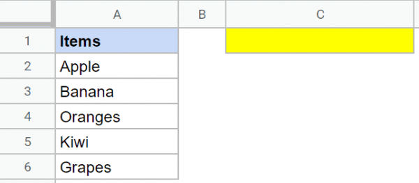
For this tutorial, we will use a dataset with the following items and create a dropdown in cell C1

To create a dropdown list that allows multiple selections, you need to do two things:

Create a dropdown list with a list of items
Add a function to the script editor that allows multiple selection in the dropdown.

Let’s take a closer look at each of these steps

Creating the drop-down list

Suppose you have a dataset of items as shown below and create a dropdown list in cell C1.

Here are the steps to do this:

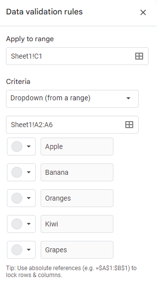
Select the cell where you want the dropdown list to appear
Go to Data > Data Validation
For Condition, select Dropdown (from range) and select the range that contains the items you want to appear in the dropdown.
Open Advanced Options and make sure Show Warning is selected instead of Reject Input (this is part of the Allow Multiple Input feature and is usually no need to do)
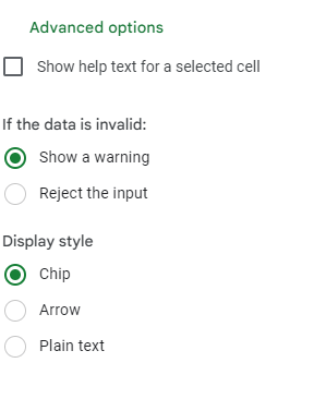
Click Save

The dropdown will now appear in the specified cell (C1 in this example). Click the arrow to see a list of options.

Please note that only one option can be selected at a time.

Next, we’ll show you how to convert this dropdown (which can only display one item in a cell) to a multiple-selection dropdown.

To do that, you’ll need to add a function script to your Google Sheets script editor.

Adding the Google Apps Script to Enable Multiple Selections

Below is the script code that you will need to copy and paste into your script editor (instructions are provided in the section after the code):

Below are the steps to add this script code to your Google Sheets backend so that you can select multiple options in the dropdown created in cell C1:

Go to Extensions > App Scripts
In the Code.gs window, delete all existing ones and copy and paste the macro code above
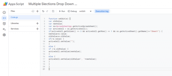
Click the Save button on the toolbar (or use the keyboard shortcut Control + S)
Click “Run

Now go back to your worksheet and try multiple selection in the dropdown. For example, first select Apple, then select Banana.

You will see that it takes 1 second (sometimes 2 seconds) and both selected items are displayed (separated by a comma).

Note: A red triangle appears in the upper right portion of the cell. It may look like an error (it’s an error because the value in the cell isn’t what you expected). You can safely ignore this.

Also note that this code allows you to select the same item twice. For example, if you select Apple and then select Apple again, Apple appears twice in the cell.

If you want to create a dropdown list that allows multiple selections without repeating, I will provide the code later in this tutorial.

how does the code work?

Let’s understand this code piece by piece.

The code starts with the line

function onEdit(e)

onEdit() is a special function in Google Sheets. Also called an event handler. This function will be triggered every time a change is made to the spreadsheet.

we want the multi-select code to run whenever an item is selected from the dropdown list, so it makes sense to put the code in the onEdit() function.

Here AppScript passes this function as an event object as an argument. The event object is usually called e. This event object contains information about the triggered event.

If you know the basics of AppScript, you’ll find the first four lines pretty straightforward:

var oldValue; var newValue; var ss=SpreadsheetApp.getActiveSpreadsheet(); var activeCell = ss.getActiveCell();

we have declared two variables. One variable holds the old value of the cell (oldValue) and the other holds the new value of the cell (newValue.

the variable activeCell holds the currently active cell that was edited.

Now you don’t need to run the code every time the cell is edited. I want it to run only if cell CA1 in Sheet1 is edited. So we use an if statement to check it:

if(activeCell.getColumn() == 3 && activeCell.getRow() == 1 && ss.getActiveSheet().getName()==”Sheet1″)

the above code checks the row and column number of the active cell as well as the sheet name. The out dropdown is in cell C1, so we check if the row number is 1 and the column number is 3.

The code inside the IF statement is executed only if all three conditions are met.

Below is the code that runs when you are in the right cell (C1 in this example)

new value=e.value; oldValue=e.oldValue;

e.oldValue is also a property of the event object. This keeps the previous value of the active cell. In this case this will be the value before making the dropdown selection

assign this to the variable oldValue.

e.value is a property of the event object. This holds the current value of the active cell. Assign this to the variable newValue.

first, let’s consider what happens when the option is not selected. In that case, e.value will be undefined. In such cases, we want cell A1 to display nothing. So put a blank value in the cell.

This is true even if the user decides to delete all previous selections and start over.

if(!e.value) { activeCell.setValue(“”); }

when the user selects an option, the lines following the else statement are executed. Here you specify what happens when an option is selected for the first time from the dropdown list.

that is, e.oldValue is undefined. In this case, we want only the selected option (newValue) to be displayed in cell A1.

if (!e.oldValue) { activeCell.setValue(newValue);

finally, specify what to do the next time the option is selected. This means that both e.value and e.oldValue hold a particular value.

else { activeCell.setValue(oldValue+’, ‘+newValue); }

After entering the code, save it and try making multiple selections from the dropdown list. All selected options are displayed one by one, separated by commas.

If you make a mistake, you can always clear the cell and start over. In this case, cell A1 should display both the previous value and the newly selected value, separated by a comma.

Note: Using the above code you cannot go back and edit part of the string. For example, you cannot manually edit the item string or remove part of it. If you want to make any changes, you will have to delete all the contents of the cell and start over.

However, there is a small problem with this. Note that selecting an item multiple times will populate the selection list again. That is, repetition is allowed. But usually we don’t want that.

Below I’ve detailed how to modify the code so that the item is selected only once and not repeated.

Allowing Multiple Selections in a Dropdown list (without repetition)

Below is the code that allows multiple selections without repetition in the dropdown.

The code above uses cell C1 of worksheet Sheet1 again as an example. If your dropdown is in a different cell (or sheet), you’ll need to adjust your code accordingly. For example, if you’re using D2, change line 6 of your code to:

if(activeCell.getColumn() == 4 && activeCell.getRow() == 2 && ss.getActiveSheet().getName()==’Sheet1′) {

D2 is the 4th column, 2nd row.

The following piece of code will allow the dropdown to ignore repeated values:

if(oldValue.indexOf(newValue) <0) { activeCell.setValue(oldValue+’, ‘+newValue); } else { activeCell.setValue(oldValue); }

here, the indexof() function checks whether the oldValue string contains the newValue string.

returns the string index of oldValue, if it exists. Otherwise, a value less than 0 is returned.

If the newly selected option is in the list, leave the list alone (so enter the previous value in cell C1). Otherwise, add the newly selected option to the list with a comma (‘, ‘) and display it in cell C1.

Multiple Selection in Drop Down (Whole Column or Multiple Cells)

The example above showed how to get a multi-select dropdown within a cell.

But what if you want to get this across columns or multiple cells.

You can easily do this with a few changes to your code.

To allow the dropdown to select multiple items across column C, we need to replace the following line of code:

if(activeCell.getColumn() == 3 && activeCell.getRow() == 1 && ss.getActiveSheet().getName()==”Sheet1″)

with the following line of code:

if(activeCell.getColumn() == 3 && ss.getActiveSheet().getName()==”Sheet1″)

When I do this, it only checks if the column is 3. All cells in Sheet1 and Column 3 satisfy this IF criteria and the dropdowns within allow multiple selection.

Similarly, if you wanted this to be available across columns C and F, use this line instead:

if(activeCell.getColumn() == 3 || 6 && ss.getActiveSheet().getName()==”Sheet1″)

Above, we use an OR condition within the IF statement to check if the column number is 3 or 6. Multiple selection is enabled if the cell with the dropdown is in column C or F.

Similarly, if you want this to work for multiple cells, you can do so by changing the code as well.

This is how you enable multiple selection in a Google Sheets dropdown. This isn’t available as a built-in feature, but it’s easy to do with the magic of Google Apps Script.

I hope you found this tutorial useful!

Want to become a Google Forms and Sheets pro? Take our masterclass!

Other Google Sheets tutorials you may find useful:

Allowing Multiple Selections in a Dropdown list (with repetition)

Creating the drop-down list

Adding the Google Apps Script to Enable Multiple Selections

Allowing Multiple Selections in a Dropdown list (without repetition)

Multiple Selection in Drop Down (Whole Column or Multiple Cells)

Related posts:

Related Posts

Leave a Comment Cancel Reply