Google Sheets Currency Conversion: Easy Guide for 2023

In this tutorial, I will show you how to perform Google Sheets Currency conversion using the GOOGLEFINANCE function.

What is the GOOGLEFINACNE Function

Working with finances can get really tricky, especially with exchange rates which are constantly changing. Luckily, Google Sheets has a convenient function called GOOGLEFINANCE, meant specifically for doing financial calculations.

The GOOGLEFINANCE function fetches real-time or historical currency information and exchange rates from the Google finance website. This saves you both the time and energy it would take to import the exchange rates from another source.

Using GOOGLEFINANCE to Convert Currency in Google Sheets

The GOOGLEFINANCE function is the perfect currency converter Google Sheets tool that fetches currency conversion rates in real-time (well almost in real-time).

You don’t need to search endless databases for the current exchange rates. All you need is the correct formula for this powerful currency converter for Google Sheets. The formula uses currency symbols to track which currency you are changing from and to.

Syntax of the GOOGLEFINANCE FUNCTION

The basic syntax of the GOOGLEFINANCE FUNCTION is as follows:

=GOOGLEFINANCE(“CURRENCY:<source_currency_symbol><target_currency_symbol>”)

where:

• source_currency_symbol is a three-letter code for the currency you want to convert from.
• target_currency_symbol is a three-letter code for the currency you want to convert to.

For example, if you want the conversion rate from dollars to rupees, you will enter the function:

=GOOGLEFINANCE(“CURRENCY:USDINR”)

Notice that there is no space between the two currency codes.

Here are some other GOOGLEFINANCE currency codes:

Currency	Code
US Dollar	USD
Japan Yen	JPY
Canada Dollar	CAD
Indian Rupee	INR
Iran Rial	IRR
Russia Ruble	RUB
Euro	EUR
Singapore Dollar	SGD
Hong Kong Dollar	HKD
United Kingdom Pound	GBP

How to Use GOOGLEFINANCE for Real-Time Currency Conversion

Let us look at an example. Here we have three currencies in column B and we want to convert currencies in column A to those in column B:

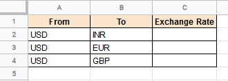
Here’s how to convert currency in Google Sheets to get the exchange rate of dollars to the three currencies in column B:

1. Select the first cell of the column where you want the results to appear (C2).
2. Type the formula: =GOOGLEFINANCE(“CURRENCY:USDINR”)
3. Press the return key.

You should see the current exchange rate for conversion of USD to INR in cell C2.

1. Alternately, you could even include references to cells in the function, by combining them with the ampersand operator, as follows: =GOOGLEFINANCE(“CURRENCY:”&A2&B2)
2. Press the return key.
3. Double click on the fill handle of cell C2 to copy the formula to the rest of the cells of column C.

You should now see conversion rates for USD to all three currencies shown in the sheet.

Note: The Google finance currency codes are the same as the shorthand codes on the international currency exchanges.

How to Convert USD to INR Using GOOGLEFINANCE

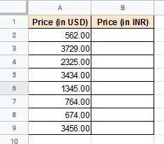
The above steps only get you the conversion rates between two currencies in Google Sheets, but they don’t actually convert money from one currency to another. Let us assume we have the following list of prices in dollars and we want to convert them to INR.

To convert the money in the table above from USD to INR, follow these steps:

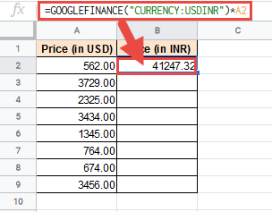
1. Select the first cell of the column where you want the results to appear (B2).
2. Type the formula: =GOOGLEFINANCE(“CURRENCY:USDINR”)*A2

   

3. Press the return key.
4. Double click on the fill handle of cell B2 to copy the formula to the rest of the cells of column C.
5. You should now see column B populated with prices in INR.
   

   

Notice we simply multiplied the result of the GOOGLEFINANCE function with the cell value in column A, in order to convert the price to INR.

Entering your parameters along with just the general GOOGLEFINANCE function is enough to give you an accurate conversion rate.

However, there are other optional parameters that the GOOGLEFINANCE function lets you enter in order to get specifically what you need. For example, you can use it to display historical exchange rates too.

Related Reading: How to Remove a Dollar Sign in Google Sheets

How to Use GOOGLE FINANCE to Fetch Historical Exchange Rates

You can make some alterations to the GOOGLEFINANCE function to fetch Google Sheet exchange rates over a period of time, instead of just one day.

To fetch historical exchange rates, the GOOGLEFINANCE function can be customized to the following syntax:

GOOGLEFINANCE(“CURRENCY:<source_currency_symbol><target_currency_symbol>”, [attribute], [start_date], [number_of_days|end_date], [interval])

Here’s an example of the formula in action. We’ll explain it further in the next section:

In the above syntax, all parameters shown in square brackets are optional. Here’s what they mean:

• The attribute parameter specifies the type of data you want to be retrieved. This is a string value and its default value is “price”. This means we want real-time price quotes fetched from Google Finance. We have provided a list of attribute values and what they mean at the end of this tutorial.
• The start_date parameter specifies the date from when we want the historical data to start
• In the fourth parameter you can either specify the end_date for the historical data or the number of days from start_date for which you want the historical data.
• The interval parameter specifies the frequency of the returned data. It can be either “DAILY” or “WEEKLY”, depending on your requirement,

How to use GOOGLEFINANCE to Fetch Currency Exchange Rates Over a Time Period

Let us take an example to understand how the GOOGLEFINANCE function can be used to fetch currency rates (USD to INR) from 10th October 2020 to 20th October 2020.

1. Select a cell from where you want to start displaying the exchange rates. You don’t need to add a header for the columns, since the function adds the column headers automatically.
2. Type the formula:=GOOGLEFINANCE(“CURRENCY:USDEUR”, “price”, DATE(2020,10,10), DATE(2020,10,20), “DAILY”)
3. Press the Return key

You should now see two new columns automatically inserted starting from the cell in which you entered the formula.

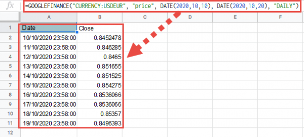
The first column contains the date for each day between 10th Oct 2020 and 20th Oct 2020. The second column contains the closing google finance exchange rate for each day.

If you want to display weekly rates instead of daily rates, you can simply replace the interval parameter in the currency conversion function from DAILY to WEEKLY.

How to use GOOGLEFINANCE to Fetch Currency Exchange Rates Over the Past Week

If you want to dynamically display exchange rates over the past, say one week depending on the day the sheet is opened, you can use the TODAY function, instead of the DATE.

Let us see an example where we want to dynamically display exchange rates of the previous 10 days, irrespective of which day the sheet is opened.

Follow these steps:

1. Select a cell from where you want to start displaying the exchange rates.
2. Type the formula: =GOOGLEFINANCE(“CURRENCY:USDEUR”, “price”, TODAY()-10, TODAY(), “DAILY”)
3. Press the Return key

You should now see two new columns automatically inserted starting from the cell in which you entered the formula.

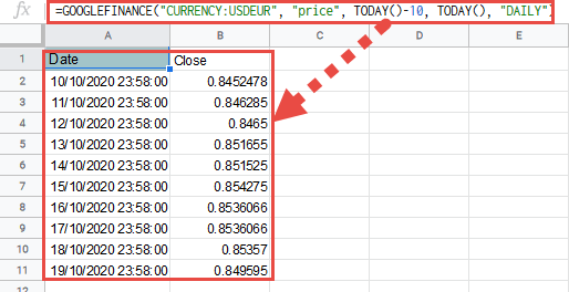
The first column contains the date for each day, from 10 days before to the current date. The second column contains the closing exchange rate for each day.

Here, the TODAY() function returns the current date on which the file is opened. So each time it is opened, this function will refresh and return a new value.

A Few Points to Remember About Google Sheet Currency Conversion

Here are a few important things you need to know to understand the GOOGLEFINANCE function:

• When we say real-time exchange rates, you can expect a delay of up to 20 minutes.
• For real-time rates, the function returns a single value. However, for historical rates, the function returns an array along with column headers.
• If you do not provide any date parameters, GOOGLEFINANCE assumes that you only want real-time results. If you provide any date parameter, the request is considered as a request for historical data.

Google Sheets Currency Conversion Attribute Values

Here are some of the commonly used values for the attribute parameter of GOOGLEFINANCE:

For real-time data:

• “priceopen” – We want the price at the time of the market open.
• “high” – We want the current day’s high price.
• “low” – We want the current day’s low price.
• “volume” – We want the current day’s trading volume.
• “marketcap” – We want the market capitalization of the stock.

For historical data:

• “open” – We want the opening price for the specified date(s).
• “close” – We want the closing price for the specified date(s).
• “high” – We want the high price for the specified date(s).
• “low” – We want the low price for the specified date(s).
• “volume” – We want the volume for the specified date(s).
• “all” – We want all the above information.

There are a number of other attributes that you can use too. You can refer to the official documentation of Google Sheets to find out more.

Google Spreadsheet Currency Conversion FAQ

Can Google Sheets Convert Currency?

Yes, You can use the GOOGLEFINACE function with the currency codes you wish to convert as the second argument like so:

=GOOGLEFINANCE(“Currency:GBPAUD”)

How Do I Convert From Pounds to Dollars in Google Sheets?

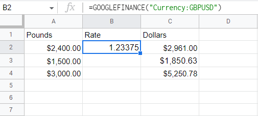
You use the GOOGLEFINANCE for currency conversions Google Sheets. You can get the current exchange rate for GBP and USD with the following formula:

=GOOGLEFINANCE(“Currency:GBPUSD”)

then multiply the two cells

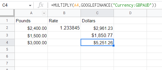
If you want to, you can convert the currency directly by combing the GOOGLEFINANCE formula with the multiply formula or asterisk sign.

In our example, you can use the formula:

=MULTIPLY(A4,GOOGLEFINANCE(“Currency:GBPAUD”))

or

=GOOGLEFINANCE(“Currency:GBPUSD”)* A4

How Do I Change Currency in Google Sheets from Pounds to Dollars?

You can also change the currency format that you are using gin Google Sheets.Here’s how to change currency in Google Sheets:

1. Highlight the cells you wish to change
2. Tap the Format > Number

3. Click Custom currencies.

4. Select the desired currency. In this case, we’ll choose dollars.

5. Click Apply.

This works for Euros or any other world currency and certain crypto coins.

How Do I Convert BTC to USD in Google Sheets?

BTC works the same as any other currency conversion using GOOGLEFINANCE in Google Sheets. You just have to use BTC the first currency argument. For example, if you just wanted the current rate, you could sue the following formula:

=GOOGLEFINANCE(“Currency:BTCUSD”)

Can I Pull Crypto Prices Into Google Sheets?

Yes, you can pull crypto prices into Google Sheets. Unfortunately, only the major cryptocurrencies are supported. For example, to pull the current exchange rate for Ethereum to USD, you could use the following formula:

=GOOGLEFINANCE(“Currency:ETHUSD”)

Is There Any Delay When GOOGLEFINANCE Fetches Values?

The Google Sheets exchange rate delay can be up to 20 minutes for the current exchange values.

Wrapping Up Google Finance Currency Conversion

In this tutorial, we looked at how you can use the GOOGLEFINANCE function to fetch both real-time and historical exchange rates.

We also looked at how you can use the fetched rates for Google Sheets Currency Conversion. We hope this has been informative and helpful for you.

Looking to upgrade your printer? We highly recommend checking out Epson’s extensive line of printers, ranging from compact and efficient home printers to large multifunction printers for your business.

Other Google Sheets tutorials you may like:

Related posts:

1. Calculate Year Over Year Growth in Excel and Google Sheets
2. How to Use HLOOKUP in Excel [An Easy 2023 Guide]
3. How to Clear Content in Google Sheets (in 2 Seconds) | SSP
4. How to Highlight Duplicates in Google Sheets 3+ Simple Ways
5. How to Make Multiple Selection in Drop-down Lists in Google Sheets
6. How to Apply a Formula to an Entire Column in Google Sheets