Contents
- 1 What is the difference between check box and checkmark in google sheets?
- 2 Insert Checkmark Using CHAR Function in google sheets?
- 3 How to add Unicode value to CHAR Function?
- 4 How to add check and cross marks as images in Google Sheets?
- 5 How to change Crossmark and checkmark in google sheets based on condition operation?
What is the difference between check box and checkmark in google sheets?

The checkbox is square boxes that are used to indicate a binary choice. In the classic checkbox return TRUE and FALSE but you can add checkboxes with custom values using conditional formatting in google sheets. This feature can execute another function & return value using checked or unchecked status.
The checkmark is the read-only icon/image or Unicode value that is used to indicate it has been dealt with in cell values such as (correct/ok / done / TRUE ). When dealing with a checkmark in google sheets, you can implement an image using the IMAGE Function or Unicode value using CHAR function also Special characters. a cross mark is the opposer of the checkmark symbol. It can be used for indicating whether a cell value is FALSE or incorrect when the checkmark indicates TRUE or Correct. this is up to the user perspective dealt in google sheets.
Let’s check how to use both Crossmark or checkmark in google sheets.
Google sheets offer a special function called CHAR Function for Converting a number into a character according to the current Unicode table. Make sure that all Unicode icons may not support google sheets. Icon colors and figures may depend on the device and font which you use.
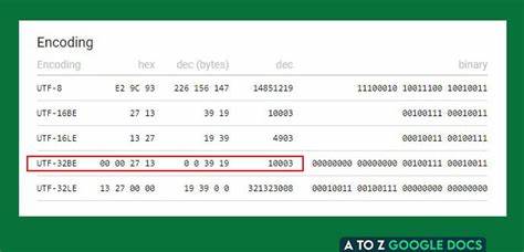
How to get Unicode value in unicode-table.com?
- search icon name on search field & then select from suggestions while you type into the field then enter.

- Then scroll down (in the icon detail page) to the Encoding section and copy the decimal value from UTF-32BE.
How to add Unicode value to CHAR Function?
After copied icon value from the current Unicode table in decimal format, then
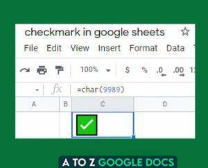
- Open a spreadsheet in Google Sheets.
- Select the cell that you want to add a Unicode value.
- Type =CHAR(add_unicode_value) in the cell then enter.
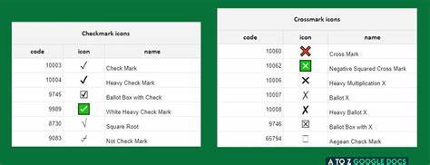
Example icon:
There are different types of checkmark and cross mark icons available in the Unicode table that are offered for your data sheet’s perspective.
How to add check and cross marks as images in Google Sheets?
Sometimes your expectation icon cannot be fulfilled from Unicode. Then you have to insert a custom icon/ image into your spreadsheet. google sheet introduces a special function for Inserts an image into a cell.
Make sure that this IMAGE function will not support SVG image and drive.google.com also not support. you can insert an image like below,
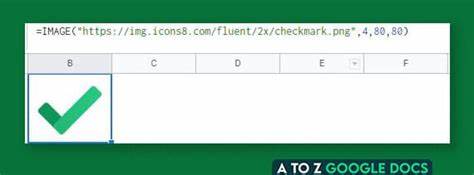
- Open a spreadsheet in Google Sheets.
- Select the cell that you want to add a IMAGE.
- Select the image you need from the external domain. including protocol (e.g. HTTP:// or HTTPS://)
- Type =IMAGE(IMAGE_URL, SIZING_MODE, HEIGHT, WIDTH) in cell then enter.
Ok, these are the most useful and useful formulas that can be imported and used to implement crossmark and checkmark in google sheets. Let’s check how to implement the condition operation.
Additionally: you can change icon color using conditional formatting in google sheets. Still don’t have any idea about how to implement conditional formatting in google sheets, we highly recommend reading the Conditional Formatting in Google Sheets ( 6 Useful Examples ) Article.
This is not big deal, I need to change the red color to Crossmark and the green color to checkmark in google sheets.
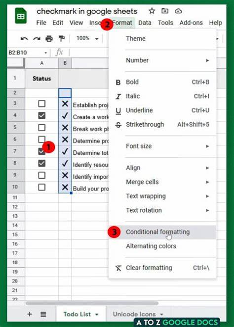
- Select column ( without row header) which exits Crossmark and checkmark in the todo list.
- On the top of the navigation click Format > Conditional Formatting.
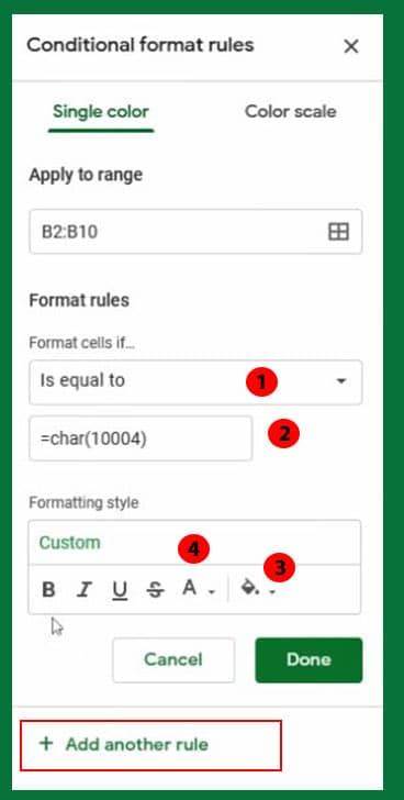
- Then select To equal to option from formula rule dropdown and add checkmark Unicode value with CHAR function into the value field. after selecting the green color and change the white background in the text style option. After click add another rule.
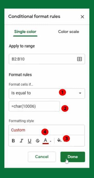
- Again select To equal to option from formula rule dropdown and add Crossmark Unicode value with CHAR function into the value field. Then select the red color and change the white background in the text style option.
- After press, the done button, above color condition applied in to the datasheet.
Please note that this color style will not support Emoji base Unicode and IMAGE Function in google sheets. also, you can implement CHAR() and IMAGE() function together with text using & syntax in google sheets. But make sure that the color conditional formatting rule will not trigger or you have to change the conditional rule based on cell value.

