7 Hottest Tips for GOOGLEFINANCE Function in Google Sheets

Google sheet isn’t just a data management tool. Its real-time web-based productivity suite allows people to work together to gather, process, and present data anytime and anywhere. GOOGLEFINANCE  is a built-in function in a google sheet that has been used to track and monitor real-time financial and currency market trends and changes, the return current or historical meaningful information from Google Finance.

This is the basic step to use the GOOGLEFINANCE function.

  1. Open a spreadsheet in Google Sheets.
  2. Select the empty cell which you want to present financial data
  3. In an empty cell, type =GOOGLEFINANCE(ticker-stock-prefix, [attribute that need to fetch from google finance], [start_date], [num_days|end_date], [interval])

GOOGLEFINANCE function in google sheets can be used for,

  1. Track and validate current stock movement and trend
  2. Analysis of major competitor performance chart.
  3. Predict future stock trends and directions based on historical data.
About This Article
In this article describe features of GOOGLEFINANCE function in google sheets and usage with different user requirements with example and how to implement different condition operation.

How to get data into GOOGLEFINANCE  function?

In google sheet using Google Finance marketplace to get financial statistics to the spreadsheet. Google finance market place is a financial information site that was started by google inc in 2006, based on Wikipedia source, in the initial stage google finance’s primary focus to provide financial decisions and major news events. After several months, they incorporated with  Stock Market(NASDAQ) and New York Stock Exchange(NYSE). Now they incorporate over 200 stock exchanges worldwide including top-level markets such as the London Stock Exchange, Hong Kong Stock Exchange, Tokyo Stock Exchange, Shanghai Stock Exchange. Google financial provides all stock exchanges, mutual funds, indexes, and other financial data.

Syntax and Features of  GOOGLEFINANCE  function in google sheets.

According to google sheet Editor’s help, the GOOGLEFINANCE  function in google sheets has the following syntax and features which allow it to be used with google sheets.
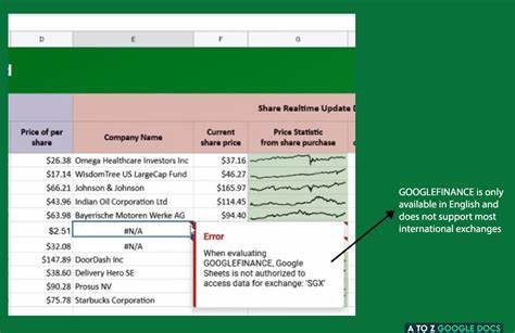
  1. tickerthe ticker is a unique identification code that is used to secure trading and updated continuously throughout the trading session by the various stock market exchanges which incorporate with google finance. This only depends on the relevant exchange market and it will duplicate with other exchange market identification.
  2. attribute:  this is the optional syntax for use to get specific trading data using ticker in google finance price is the default. some attributes may not emit results for all symbols even if a ticker is allowed. Click to discover all attributes in GOOGLEFINANCE Function.Real-time results will be returned as a value within a single cell & t may be delayed up to 20 minutes so far.
  3. start_date :    this is the optional syntax that is used to get historical data in ticker from google sheets.
  4. end_date| num_days:  this is also an optional syntax that is used to get historical data from google finance for the specific period based on the start date. In num_day syntax use for day count from the start date.
  5. interval – this is the optional syntax that uses a set frequency of returned data; either “DAILY” / “1” or “WEEKLY” / “7”.

About example

One of your clients who is a medium-level share market investor was purchasing various companies’ shares in various exchange markets. He doesn’t have time to invest in a computer and check each exchange market behavior. Then he consulted me to create a real-time web-based productivity data sheet to track and summarize each share’s behavior in the primer exchange market. He shared,

To Import the example datasheet into your spreadsheet,

  1. Open a spreadsheet in Google Sheets.
  2. On the top of navigation click File > Import (import datasheet)

Let’s continue all our particle topics based on the above example datasheet.

Get company name base on Ticker

In E column l in Google Sheets need to fill the corporate name base on column (ticker). In attribute called “name” to use with GOOGLEFINANCE function in google sheets, to fetch the corporate name.

=GOOGLEFINANCE(A4,"name")


To apply for all cells in column E, select E4 cell then click the square icon in the bottom right then drag till the last cell which data exits.

NOTE: Still GOOGLEFINANCE in google sheets will only support English and most of the international exchange’s data may not return even google finance exit. Following exchanges market will not support in google sheets TYO, INDEXTYO, BKK, INDEXBKK, SHA, INDEXCSI, SGX, & KLSE.


Get the latest share price quote  on Ticker

Google sheet enables to get real-time update data up to 20-minute delay. In an attribute called “price” take each ticker’s latest price quote in the USD default currency. In our example, the F column defines all ticker price quotes.

=GOOGLEFINANCE(A4, "price")


To apply for all cells in column F, select the F4 cell then click the square icon in the bottom right then drag till the last cell which data exits.

NOTE: price will return as default number format to apply a currency format.  Select cell > On the top of navigation click Format Number Currency


How to get the shape of the variation in share behavior from purchase date?

Practically You cannot check each day’s market variant in your spreadsheet. Instead of text data, graphic static charts will be suitable to do that. I decided to implement sparkline in google sheets to get historical share data as a line chart. We have to combine multiple functions together with the GOOGLEFINANCE function in google sheets.


To access the graphical interface in price variant we have to list historical prices from purchase date.

Still don’t have any idea about logical operators in google sheets, we highly recommend reading How To Format Date In Google Sheets  Article.

Our client needs to put all historical price statistics onto a miniature chart from the purchased date to today. In the C column exit all purchase date history which purchases a share in the exchange market.

=SPARKLINE(GOOGLEFINANCE(A4, "price", C4, TODAY()))

In column G use for defined all Price Statistic from share purchase.


Now you can get a miniature chart of each ticker price variant from the purchase date to the current date. You can modify the color of a line chart, change the font color of the cell using sparklink formula syntax


How do get prices change from the last trading date?

When getting a trading decision stock price statistics are important. We can use changepct syntax in GOOGLEFINANCE function to return the price since the previous trading day’s close. to get the percentage, the return value can be divided by 100.

=GOOGLEFINANCE(A4, "changepct")/100


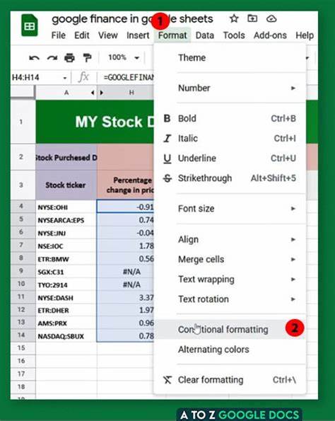
So I need to apply the % symbol to change price variants. I need to show less than zero(0) results as red color and greater than zero(0) results as green color.

  1. Select H column cell range (H4:H14)
  2. On the top of the navigation click Format Number More Formats > Custom Number format.
  3. Enter 0.000% in the custom number format dialog box and click apply. Then changepct return value will be shown with the % symbol.
  4. Next again select the H column cell range (H4:H14)  and click the top of navigation click Format Conditional formatting.
  5. Next in the conditional formatting dialog box, select greater than option from format rule and enter zero (0) in the Value field, then change background color to white and change the text color for green.then click Add another rule and change format rule to less than. Next enter zero (0) in the Value field, then change the background color to white and change the text color for red. Then click or button.
    Still don’t have any idea about logical operators in google sheets, we highly recommend reading Conditional Formatting in Google Sheets – 6 Useful Examples –  In Google Sheets  Article.
  6. Then  Percentage change in price will appear on the sheet clearly.


How to get earnings per share from the last trading date?

In the trading market earning per share is calculated as a company profit divided by the outstanding shares of its common stock (ref: Earnings Per Share (EPS)). In googlefinance use an attribute called “eps” to get The earnings per share base on the ticker./ it will recalculate as real-time data. In Column, I use to fetch all EPS value trading data.

=GOOGLEFINANCE(A4, "eps")

In Column I use to get all company share outstanding base on ticker.

NOTE: price will return as default number format to apply a currency format

Select cell > On the top of navigation click Format Number Currency

To apply for all cells in column I, select I4 cell then click the square icon in the bottom right then drag till the last cell which data exit.


How to get the total number of shares issued?

Outstanding shares ratio important to get an understanding of variables in financial ratios, making them important for fundamental analysis. In googlefinance uses an attribute called “shares” to get a company’s shares outstanding.

=GOOGLEFINANCE(A4,"shares")

Column J use to get all company share outstanding base on the ticker

To apply for all cells in column J, select the J4 cell then click the square icon in the bottom right then drag till the last row which data exit.

You can see that this number cannot be read clearly. For huge numbers, it is easier to read group numbers to m in showcase abbreviated numbers. Let’s check how to convert in google sheets.

  1. Select H column cell range (J4:J14)
  2. On the top of the navigation click Format > Number > More Formats > Custom Number format.
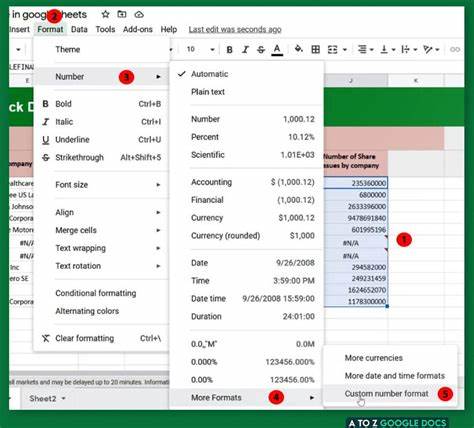
  3. If you would like to see 23.6M, you can insert to 0.0,,”M” into the custom format field and click apply.
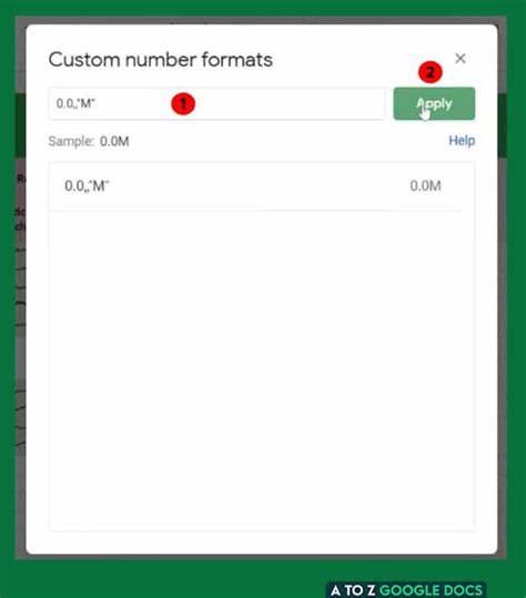
    Shares count will arrange Million Suffix.

Error Handling in GOOGLEFINANCE  function.

When you work with data you have to face different types corresponding to error values. It very in google Sheets uses a formula called  IFERROR() to check whether a value is an error. This function is most often used in conjunction with IF in the conditional statement.

Let’s check how to implement with GOOGLEFINANCE  function in google sheets.


The above error will appear if you try to get trading data from unsupported international exchanges in google sheets. To give the meaningful message, we can conjunction IFERROR() with GOOGLEFINANCE  function in google sheets.

=IFERROR(GOOGLEFINANCE(A4,"name"),"Not Authorized to Access data")


Still don’t have any idea about conditional function in google sheets, we highly recommend reading Right Way To Use Google Sheets IF Function ( With 6 Helpful Tips ) In Google Sheets  Article.

Ok, this is the basic implementation of the GOOGLEFINANCE  function in google sheets. Hope this tutorial can help you to get a basic idea about google finance syntax handling within Google Sheets Enjoy!

Conclusion

Google sheets is an extremely powerful software and it works with many subsidiary tools in google have. Google Finance is one of the most usable platforms in the trading industry. Many stakeholders are using that platform to get financial statistics & make decisions. This is  one place platform that incorporates over 200 exchange markets world-wide. Google sheet introduces GOOGLEFINANCE function to collaborate with google finance trading data to get most of trading related data into your spreadsheets.

Scroll to Top